Network analysis using the ladder method
October 18, 2025 - Reading time: 11 minutes
If you're looking to find a way of working out the transfer function of a complicated network, or want to find out the voltages and currents in that network, the ladder method may be of interest. The beauty of this method is the breaking down of the problem into small manageable steps.
Consider the schematic of a pi-network below:
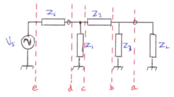
We first draw lines separating the individual components, or 'planes'. We work backwards from the load, calculating either the admittance or the impedance, dependent on whether the next component is in shunt or series. When we have finally got to the source, we have a number of admittance and impedance expressions that only need to be multiplied together to obtain the transfer function. This may be proved by nodal analysis working in the other direction, from front to back:

Notice that if we had no Zs we would have started with a current (Id). This is convenient if we want to know the transimpedance. I have used this method to analyse some fairly complicated charge pump PLL loop filters, for example.
I've analysed a pi-network, but you can see how the method can be extended to an arbitrary ladder length.
The method is best illustrated with an example. Here I've used Octave, an open source alternative to Matlab - a scientific programming language. This means you don't have to do any complex number arithmetic. However, the method is quite amenable to hand calculation if you want to. Each step involves finding the reciprocal of a complex number, which can be achieved by conversion from cartesian to polar format, finding the reciprocal of the magnitude and inverting the sign of the angle. You will also need to be able to convert back to cartesian format. I'll leave you to Google how to do the format conversion. Alternatively, download Octave and run this file:
You can edit the file for your particular needs. Note that any of the impedances can be set to 'inf' or 0 to create open or short-circuits. This allows L-networks to be analysed.
Here I've pasted what's in Ladder1.m, so you can see what it does. Sorry about the lack of syntax highlighting! At the bottom, I've pasted the output from it. I've included some other commented-out examples of a 3dB resistive pad, and a 30MHz Butterworth low-pass filter, to illustrate how to enter component values.
Happy analysing!
Ladder1.m
% A calculator of voltages and currents in a pi-network, using the ladder method of network analysis.
% Shunt components can be ignored by setting to inf. Series components can be ignored by setting to 0;
% Inductances are always 1j*w*L.
% Capacitances are always 1./(1j*w*C).
clear all;
close all;
% Use the spot frequency to allow display of voltages and currents at the command line.
f_spot = 10.125e6;
f = [f_spot, logspace(5, 8, 1000)]; % 10^5Hz to 10^8Hz, 1000 points, with a custom spot frequency.
w = 2.*pi.*f;
% Example matching network at f_spot.
ZS = 50;
Z1 = inf;
Z2 = 1./(1j*w*145e-12); % i.e. a 145pF capacitor.
Z3 = 0.47+ 1j*w*1.1e-6; % i.e a 1.1uH inductor with a Q of 150 @10.125MHz (Rs = wL/Q).
ZL = 64 - 1j*119;
% Example 3dB pad.
%ZS = 50;
%Z1 = 292;
%Z2 = 17.6;
%Z3 = 292;
%ZL = 50;
% Example 30MHz cut-off Butterworth low-pass filter.
%ZS = 50;
%Z1 = 1./(1j*w*106e-12);
%Z2 = 1j*w*375e-9;
%Z3 = 1./(1j*w*106e-12);
%ZL = 50;
Ps = 400; % Power in watts.
Vs = 2.*sqrt(Ps.*ZS); % [rms] The emf is twice the voltage developed across its conjugate.
% The process involves first calculating the immittances at each plane, starting from the load and working backwards.
% The first component we see is in shunt, so we convert ZL to admittance, which is also the admittance looking into
% plane a from left to right:
YL = 1./ZL;
% We also need Z3 expressed as an admittance, so that we can combine them simply by adding:
Y3 = 1./Z3;
% The summation of Y3 with YL is the admittance looking into plane b from left to right:
Yb = Y3 + YL;
% The next component is in series, so we must first convert Yb to impedance:
Zb = 1./Yb;
% The summation of Z2 with Zb is the impedance looking into plane c from left to right:
Zc = Z2 + Zb;
% The next component is in shunt, so we must first convert Zc to admittance:
Yc = 1./Zc;
% We also need Z1 expressed as an admittance:
Y1 = 1./Z1;
% The summation of Y1 with Yc is the impedance looking into plane d from left to right:
Yd = Y1 + Yc;
% The next component is in series, so we must first convert Yd to impedance:
Zd = 1./Yd;
% The summation of ZS with Zd is the impedance looking into plane e from left to right:
Ze = ZS + Zd;
% We will also need this expressed as an admittance:
Ye = 1./Ze;
% Now that we have calculated the immittances at each plane, we can work out the node voltages and currents.
% The current flowing into plane e from left to right is:
Ie = Vs./Ze;
% Which is also the current flowing into plane d from left to right:
Id = Ie;
% The voltage at plane d is then:
Vd = Id.*Zd;
% Which is also equal to the voltage at plane c:
Vc = Vd;
% The current flowing into plane c from left to right is:
Ic = Vc./Zc;
% Which is also the current flowing into plane b from left to right:
Ib = Ic;
% The voltage at plane b is then:
Vb = Ib.*Zb;
% Which is also equal to the voltage at plane a (the load).
Va = Vb;
VL = Va;
% The load current is then:
IL = VL./ZL;
% We may also want to know the voltage developed across Z2, i.e. between planes c & b:
VZ2 = Vc - Vb;
% And we may also want to know the current flowing in Z1 & Z2:
IZ1 = Id - Ic;
IZ3 = Ib - IL;
% It's probably more convenient to express the working voltages and currents in polar form:
[VZ1_ang, VZ1_mag] = cart2pol(real(Vd), imag(Vd));
[IZ1_ang, IZ1_mag] = cart2pol(real(IZ1), imag(IZ1));
[VZ2_ang, VZ2_mag] = cart2pol(real(VZ2), imag(VZ2));
[IZ2_ang, IZ2_mag] = cart2pol(real(Ic), imag(Ic));
[VZ3_ang, VZ3_mag] = cart2pol(real(Vb), imag(Vb));
[IZ3_ang, IZ3_mag] = cart2pol(real(IZ3), imag(IZ3));
% Let's print the voltages and currents to the command line:
fprintf('At f = %gHz, with %0.1fW applied\n', f_spot, 400);
fprintf('Input Z = (%0.2f + j%0.2f)Ohms\n', real(Zd(1)), imag(Zd(1)));
fprintf('Z1 voltage = %0.2fVrms /_ %0.1f deg, Z1 current = %0.2fArms /_ %0.1f deg\n', VZ1_mag(1), VZ1_ang(1).*180./pi, IZ1_mag(1), IZ1_ang(1).*180./pi);
fprintf('Z2 voltage = %0.2fVrms /_ %0.1f deg, Z2 current = %0.2fArms /_ %0.1f deg\n', VZ2_mag(1), VZ2_ang(1).*180./pi, IZ2_mag(1), IZ2_ang(1).*180./pi);
fprintf('Z3 voltage = %0.2fVrms /_ %0.1f deg, Z3 current = %0.2fArms /_ %0.1f deg\n', VZ3_mag(1), VZ3_ang(1).*180./pi, IZ3_mag(1), IZ3_ang(1).*180./pi);
% By substitution of the appropriate equations above, it is possible to determine that the transfer function is given by:
H = Zb .* Yc .* Zd .* Ye;
% We can plot this transfer function (Note the factor of two for transducer gain).
% If the load is reactive, e.g. this is a matching network, note that this won't give us the transfer function for what is delivered to the real part of the load.
semilogx(f(2:end), 20*log10(abs(2.*H(2:end))));
xlabel('freq [Hz]');
ylabel('Magnitude [dB]');
grid on;