Broadband Rx active loop antennas

October 18, 2025 - Reading time: 24 minutes

This page is a 'work in progress'. It catalogues my interest in receive only broadband active loop antennas.

Loop antenna theory

According to Faraday's law of induction, a time varying magnetic field gives rise to an induced emf in a closed loop of wire. The magnitude of that voltage depends on the strength (density) of the magnetic flux that the loop encloses, and therefore also the area of the loop (A). For a given length of wire, the area is maximised by using a circular loop. Adding more turns (N) in series increases the voltage in proportion.

What's not so obvious from Faraday's equation is that the rate of change of flux corresponds to the signal frequency, and so the voltage magnitude increases in proportion to frequency.

In addition, for a given magnetic field strength (H), the magnetic flux density (B) depends on the medium's permeability. Typically, we reference the permeability to that of a vacuum, using relative permeability. This accounts for the increased sensitivity that a high relative permeability ferrite rod imparts to a simple AM radio.

These observations are encapsulated in the following equation describing the magnitude of the induced voltage:

Where v and H are rms quantities.

An unavoidable consequence of making a loop of wire is that it possesses inductance. There's a good overview of appropriate formulas at http://www.qsl.net/in3otd/rlsim.html. A formula attributed to Grover for a single rectangular loop (FW Grover, "Inductance Calculations: Working Formulas and Tables", D Van Nostrand Co., New York, 1946) is shown below:



Where a and b are the length of the sides and d is the wire diameter (all in meters).

We also have some resistance attributable to radiation resistance and loss. And we also have some stray capacitance (which might be large if the loop has an electrostatic shield).

So the Thevenin equivalent circuit is as shown below:



If we were to resonate the loop, by adding capacitance in parallel to Ca such that the capacitive reactance (X_Ca) equals the inductive reactance (X_La) at the frequency of interest, the current that flows is limited only by Ra. The voltage developed across Ca (assuming an infinite load resistance) is that current multiplied by X_Ca. Thus voltage 'magnification' of Va occurs through the ratio X_Ca/Ra, which is the definition of quality factor (Q). More commonly, since X_Ca=X_La, and Q tends to be dominated by inductive losses, Q is defined as Q = X_La/Ra.

In practice, large values of Q are required if active amplification is to be avoided, which results in narrow bandwidth. At low operating frequencies it might even compromise speech bandwidth!

Of more interest in broadband loops is the Norton equivalent circuit. The impedance seen at the terminating port is obtained by removing the voltage source above and replacing it with a short-circuit. The current (Ia) is obtained by shorting the output and calculating the current that flows, i.e. Ia = Va/(Ra + X_La). Notice that X_Ca does not appear in the equation because it has been shorted-out. The resulting Norton equivalent circuit is shown below:

If the output current is sensed in an ideal short-circuit termination, all of the current must flow through this termination and not through La, Ra, or Ca (hence the calculation of Ia above). Remember that Va ∝ f, and since X_La dominates, which is also ∝ f, Ia is flat with frequency!

So what happens if the termination isn't an ideal short circuit? To simplify the analysis we shall separately consider the high frequency response and the low frequency response, the total frequency response being the superposition of the two. Furthermore, it will be assumed that La >> Ra, so that we can ignore Ra. Clearly, at infinite frequency Ca shorts all the available current, whereas at DC La shorts all the available current. Thus we have two circuits to solve with termination Rt:



To determine the frequency response, we need to calculate the ratio It/Ia in each case. Since Ia divides according to the branch conductances, and using Laplace notation:

        &        

Simplifying and making It/Ia the subject of the formula:

        &         

Since s = jω, the -3dB corner frequencies occur when the imaginary part equals the real part (i.e. √(1²+1²)). It can therefore be shown that:

        &        

So to maximise the high frequency bandwidth we must reduce stray capacitance (Ca) and strive for low termination resistance (Rt). If high frequency bandwidth is important, it's probably not a good idea to use an electrostatic shield.

To maximise low frequency bandwidth, which is the most likely scenario, we also need low termination resistance, but we also need large inductance (La). This may seem perverse, given that earlier we showed that Ia is principally limited by the reactance of La! What this says is that for a given Rt the low frequency sensed output current is controlled solely by La (reducing it is better), but that at progressively higher frequencies more output can be obtained, depending on the ratio of Rt/La. Put another way, if low frequency response flatness is important to you then you may have to sacrifice absolute sensitivity. Of course, the nicest solution would be to achieve low enough Rt for your particular loop to set the corner frequency at the lowest frequency of interest.

Let's consider an example. I'm principally interested in 1.8 ~ 30MHz. If I re-use the single band 80m loop data (UR43 square loop, 0.9mm centre conductor, 0.76m sides) I have a loop inductance of 4.1uH, and the centre-to-braid capacitance is 152pF. For a lower -3dB frequency of 1.8MHz, Rt = 46Ω. With this termination resistance, the upper -3dB frequency would be 22.8MHz. If I really want operation up to 30MHz I might need to abandon using an electrostatic shield, although at these frequencies the loop is getting electrically too large to operate in a 'small loop' manner anyway.

We said that the output would scale proportionate to the number of turns in the loop. Unfortunately, La scales according to N², so the net effect would be to halve the current for a doubling of N. In the case where the loop is resonated, the voltage would be proportional to N, but the Q would increase in proportion to N². This explains why you don't see multi-turn loops used where the current is sensed. Reducing La will increase the output in proportion, so we need to strive for a smaller La without reducing the loop area. This steers us towards a loop conductor that is wide and thin.

Needed sensitivity

The above begs the question as to what loop sensitivity is necessary, and therefore what loop parameters are needed. This is more a question of SNR. Radiation resistance does not generate Johnson noise like a resistor would, so in practice SNR is limited only by Rt. We need to know whether background noise exceeds the Johnson noise in Rt.

The classic CCIR Report 322 gave us information on background radio noise. This has now been superseded by ITU-R P.372, which is very similar. At the time of writing, version 17 (08/2024) was publicly available here. Part 6 of this document gives formulas for expected man-made noise, for categorised environments. Part 7 presents plots for atmospheric noise at various percentiles, for each season and in 4 hourly intervals. I extracted the 50th percentile data (i.e. the mean) for spring 12:00-16:00 (day) and 20:00-24:00 (night). The data is plotted below:

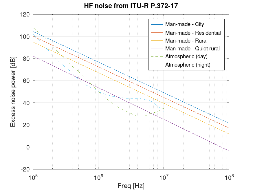
The y-axis is the excess noise power relative to kTB, i.e. the effective noise figure. P.372-17 says a short monopole was used to measure the noise power, and in Part 1 an equation is given to convert the excess noise power to electric field strength in a given bandwidth (as dBuV/m). The above plot may therefore be converted to this quantity:

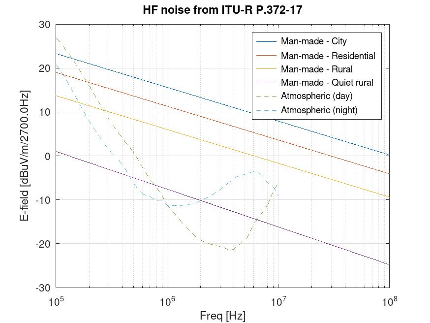
Here I've used 2.7kHz bandwidth for comparison with these same curves plotted by VERON here, to check my maths. The RSGB also have a leaflet here. They've clearly used a different noise bandwidth, but they haven't said what this is. It looks like 9kHz was used. I don't know what atmospheric data was used in the RSGB leaflet. They claim 'UK day' and 'UK night', but P.372 gives worldwide data. The VERON presentation shows 20th, 50th and 80th percentile curves, but it's not clear which season and time of day was used. The upshot is that I think you can take any of these curves (mine included) as a guide, rather than fact. Probably, a higher percentile curve should be used for night time atmospheric noise, so that curve should probably be higher, especially at lower frequencies.

We need to know the magnetic field strength to calculate the induced loop voltage. This is related via the impedance of free-space (377R or 120*pi), so it's the same plot but with a different y-axis:

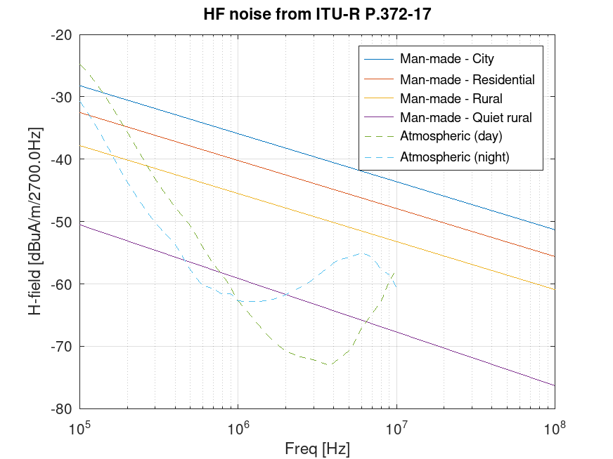
Using Octave, I calculate the transfer function of current in the termination resistance to magnetic field strength stimulus, and I can use the curves generated in the plot above as the stimulus. The plot below uses a 0.76m sided square loop with 4uH inductance and only 10pF shunt capacitance (so plain wire, not RG58). A termination resistance of 5R is used.

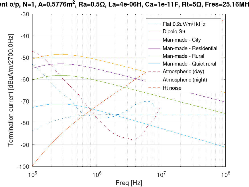
Sorry about the cropped the title. This is a busy plot, so needs some explanation.

LZ1AQ uses a flat 0.2uV/m/1kHz as a background noise level in his loop antenna work, saying that it represents a quiet rural environment. I've renormalised this value for 2.7kHz bandwidth in the above plot. You can see that it is indeed a fair representation of both the quiet rural curve and the atmospheric data from P.372. It's also useful to plot the output with a flat magnetic field strength over frequency to see the loop's uncoloured transfer function. For later reference purposes, this noise level works out as 3pA/sqrt(Hz), for these particular loop parameters.

To get some perspective, the magnetic field strength needed for a dipole in free space to receive an S9 (50uV) signal was calculated, and this was also passed through the loop transfer function.

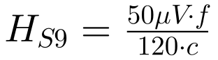
Where c is the speed of light. It's interesting that for example at 4MHz, quiet rural noise is only about 19dB down on S9 in 2.7kHz bandwidth. With 6dB per S-unit, that would suggest the noise would be sitting a bit below S6. I'm not sure I believe that!

The bad news is that the termination resistance generates Johnson noise. The RMS noise current in bandwidth B is given by:

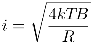
This noise level is shown in the above plot. The implication is that we wouldn't even hear an S9 signal at 4MHz! How can this be the case?  In fact, and ignoring other effects, to get down to the noise floor LZ1AQ recommends would require the resistor to be about 400 times larger. The signal current is dominated by the loop's inductive reactance, so increasing Rt does improve SNR. The disadvantage is that the lower corner frequency increases (as noted previously). For obvious reasons, it's instructive to plot the result with 50R termination:

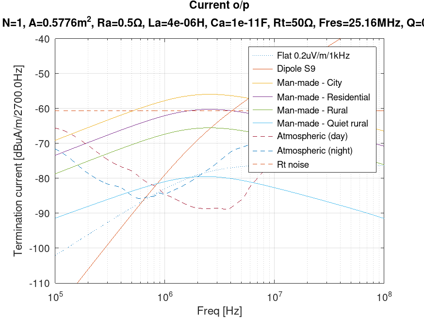
The gap between the background noise target and Rt noise has been closed by nearly 10dB compared to the previous plot (@4MHz), but at the expense of LF roll-off.

The KC2TX design referenced in single band 80m loop can also be accommodated in this model. The termination is 200R (not 50R), and the loop is resonated:

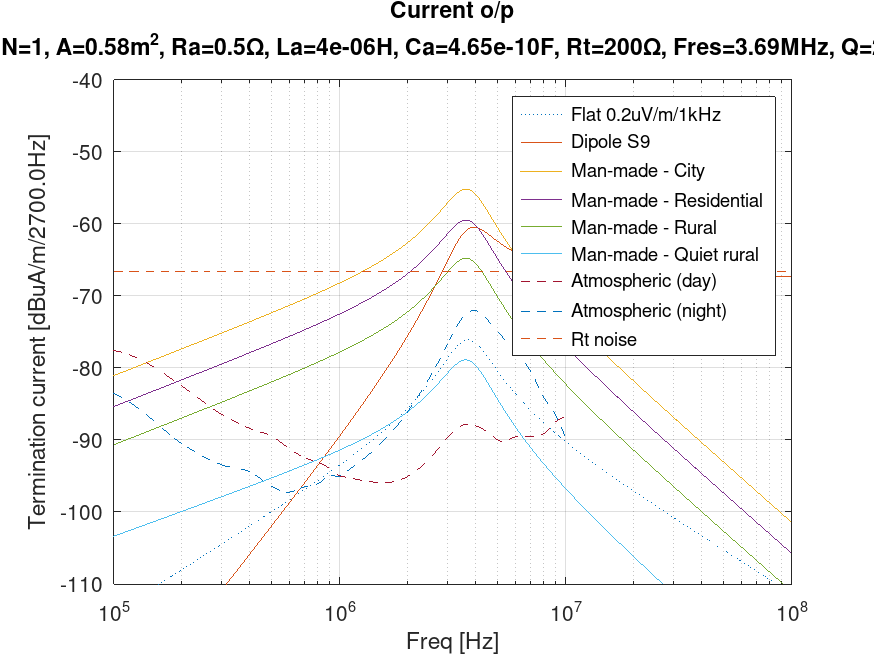
The gap to the target is now only about 10dB, but we are already bettering rural man-made noise. Some of that benefit is the increase to 200R, and some of it is the increase in signal voltage across Rt due to resonance (it's been cropped off the title, but the Q was 2.2 at resonance). Note that we could take the output as voltage instead - it's the same set of curves scaled by Rt.

Going a bit further, in my design described in single band 80m loop I terminate the loop in 1.12k:

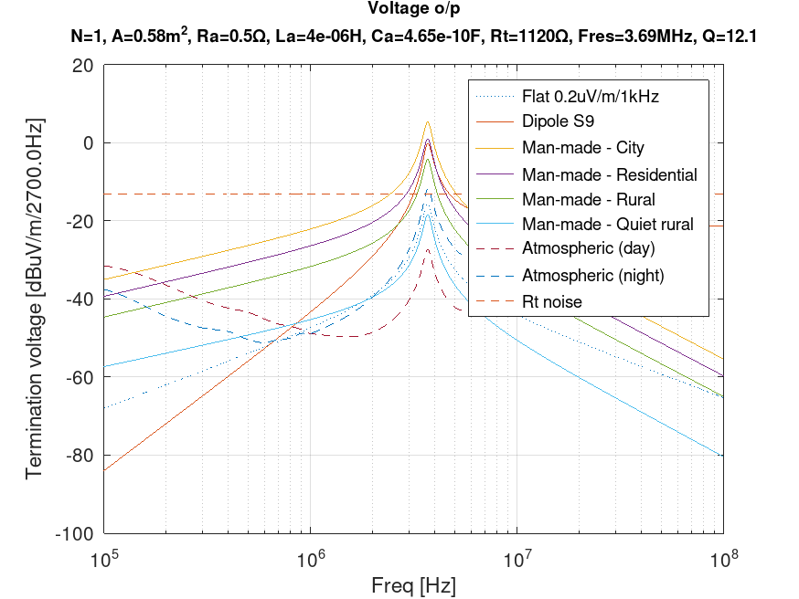
Here I've switched to voltage output for demonstration purposes, and I seem to have got all the title text on screen this time!

We're now within a few dBs of the target. If the loop's side length was doubled, the inductance works out as about 9uH. Re-resonating with 200pF would get us down to quiet rural with a Q of 5.5. Of course, none of this takes into consideration the noise of the active pre-amp, but it could all be done with passive transformers. The general take-away is that sensitivity can be traded for Q. It's not surprising that more success has been had with resonated loops in the past.

 The magic of the trans-impedance amplifier

Consider the op-amp based trans-impedance amplifier, commonly abbreviated to TIA:

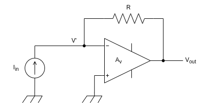
         (1)

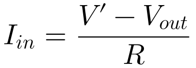          (2)

Substituting (1) into (2) and solving for Vout:

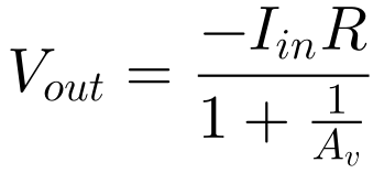             (3)

For large Av, the denominator becomes unity. We have an ideal current to voltage converter. Of course, we could have done that with just the resistor, but the TIA is more like an ideal current-controlled voltage source, in as much as we want the input resistance to be zero. Here, the input resistance is simply:

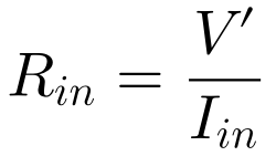
Substituting (1) and (3) into this formula, we get:

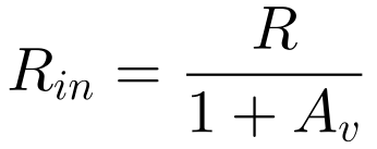
So the input resistance is R reduced by a 1+Av factor. For large Av, Rin -> 0.

What's even more useful in our application is that the Johnson noise voltage from R appears at the output with unity gain. We get a loop termination that is vanishingly small, but without it's noise penalty. One way of thinking about this is that the noise current from R flows in series with the source, so the loop termination sees the noise current from a much larger resistor, despite Rt appearing much smaller. We know that 1.12k was pretty good. In fact, 2k would get us down to LZ1AQ's target. We also know that 5R termination resistance gives an acceptable lower corner frequency for the loop size chosen. That implies that we need Av = 2k/5 - 1 = 399. That's still quite large (52dB), but possible in a wideband op-amp.

One aspect to be careful of is capacitance at the op-amp input. This causes phase shift in the feedback path, which can cause peaking in the voltage transfer function from the input. That can severely degrade the noise performance at higher frequencies due to the op-amp's input noise voltage (as opposed to its input noise current).

Op-amps aren't mandatory. Use can be made of feedback in discrete solutions.

References

https://sidstation.loudet.org/antenna-theory-en.xhtml

https://www.lz1aq.signacor.com/docs/fa-eng/Weak_signals-mag_loop_engl.htm

https://www.lz1aq.signacor.com/docs/wsml/wideband-active-sm-loop-antenna.htm